Recently, there has been a lot of buzz around Large Language Models (LLMs) (opens new window) and their diverse use cases, from chatbots (opens new window) to content generation. However, despite their multiple applications, LLMs face significant challenges in real-world deployment, particularly when it comes to running efficiently on different hardware devices. These models are computationally heavy and require substantial memory, making it difficult to run them on devices with limited processing capabilities like smartphones and tablets. This limitation can hinder the widespread adoption of LLMs.
To address these challenges, researchers have introduced quantization as a viable solution. Quantization reduces a model's memory usage and size, enabling it to run on different devices without sacrificing performance by converting high-precision parameters to lower-precision formats.
In this article, we will delve into the principles of LLMs, their transformative impact on NLP tasks, and the critical need for optimizing these models for diverse hardware platforms. We will also address the optimization challenges and highlight quantization as a powerful method for deploying LLMs across various devices.
# How LLMs Work and the Need for Quantization
LLMs operate by training on vast datasets that include books, articles, and web content. They learn to understand and generate human language by adjusting millions or even billions of parameters, which are essentially weights that the model fine-tunes during training to minimize prediction errors. These weights take up substantial memory, which can be a significant challenge for devices with limited computational resources.
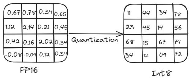
For instance, a model with 5 billion parameters requires around 10 GB of memory to load when using 16-bit precision, making it impractical for devices with limited computational capabilities. This is where quantization becomes essential. By reducing the precision of the model's parameters, quantization decreases memory usage and computational load without significantly compromising performance. This process involves converting high-precision weights and activations (e.g., 16-bit floating point or 32-bit floating) to lower precision (e.g., 8-bit integer).
# Overview of Quantization:
Quantization is crucial for deploying LLMs efficiently on various hardware platforms. It reduces model size and computational demands by converting high-precision weights and activations (e.g., 32-bit floating point) to lower precision (e.g., 8-bit integer). This reduction in precision leads to smaller model sizes, faster computation, and lower memory usage, making it feasible to run models on edge devices like smartphones and IoT devices without significant loss in accuracy.

Quantization process
# How Quantization is Performed?
Quantization can be performed using two main methods: symmetric and asymmetric quantization.
# Symmetric Quantization
This approach scales both positive and negative values symmetrically around zero. The same scale factor is used for all values, simplifying computations but sometimes resulting in less efficient representation for values with a skewed distribution.
Imagine we have a range of floating-point numbers from -6 to 5. To quantize these values, we find the maximum absolute value, which is 6. We use this value to scale the entire range. In an 8-bit representation, the range is from -128 to 127. So, we map -6 to -128, 0 to 0, and 5 to about 106. This way, the scaling is symmetric around zero.
Q=round(SX)
Here, S is the scale factor (e.g., 6/128).
# Asymmetric Quantization
This method uses different scale factors for different ranges of values. It provides more flexibility and often results in better model performance but can be more complex to implement.
Suppose we have a range of floating-point numbers from 0 to 10. In an 8-bit representation, this range can be mapped directly to 0 to 255, utilizing the entire range of quantized values. Here, zero-point is used to align the ranges properly, ensuring the entire range is used efficiently.
X=Q×S+Z
Here,S is the scale factor, and Z is the zero-point adjustment.
# Modes of Quantization
There are two primary modes of quantization: post-training quantization and quantization-aware training.
# Post-Training Quantization (PTQ)
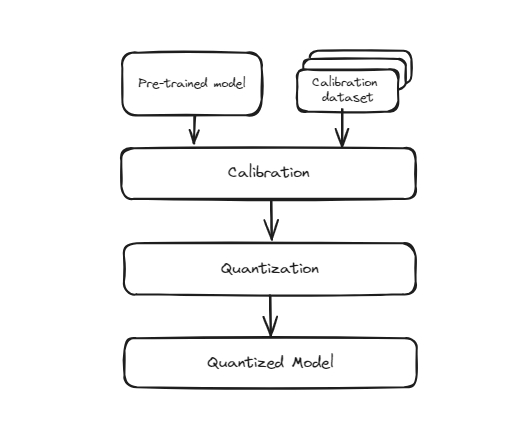
This method involves taking a model that has already been trained with full precision (usually in 32-bit floating-point) and converting it to a lower precision format (such as 8-bit integers) after the training is complete. The process is straightforward and quick because it doesn't require retraining the model. However, since the model wasn't originally trained to operate at this lower precision, there's a chance that its accuracy might slightly decrease. This is because the model's weights and activations are approximated to fit into the smaller bit representation, which can introduce some quantization errors.

Pre Training Quantization
However, during this conversion, the precision of the weights is reduced, which might lead to a slight drop in the model's performance in recognizing digits accurately. It is especially useful in scenarios where model size and inference speed are critical, such as mobile applications, embedded systems, and edge computing. Despite the potential slight drop in accuracy, the trade-offs are often worth it for the benefits of efficiency and scalability.
# Quantization-Aware Training (QAT)
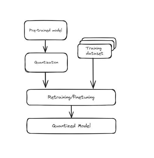
This technique incorporates quantization directly into the training process of the neural network. Instead of training the model first and then converting it to a lower precision, QAT trains the model while considering the lower precision from the beginning. This means that during training, the model's weights and activations are "fake quantized" to simulate the effects of lower precision. This helps the model learn how to operate effectively within the constraints of quantized values, leading to better performance when actually converted to lower precision. QAT requires more computational resources and time since the model undergoes additional steps during training, but it typically results in higher accuracy compared to Post-Training Quantization (PTQ).

Training Aware Quantization
It’s particularly useful for applications where maintaining high accuracy is crucial, such as in image recognition, natural language processing, and other AI tasks. Despite the increased training time and resource requirements, the improved performance and accuracy at lower precision make QAT a valuable technique for deploying high-performing models in resource-constrained environments.
# Pros and Cons of Quantization
Pros:
- Models take up less storage space, making them easier to distribute and deploy.
- Lower precision computations are faster, improving real-time performance.
- Ideal for battery-powered devices.
Cons:
- Quantization can introduce errors, reducing model accuracy.
- Especially for asymmetric quantization and QAT.
- Not all hardware supports all types of quantization efficiently.
# Practical Example of Quantization
In this example, we will demonstrate how to perform dynamic quantization on a pre-trained DistilBERT model using the transformers and torch libraries. This will help reduce the model size and make it suitable for deployment on devices with limited computational resources.
Let's create a Python script to load a pre-trained DistilBERT model, perform dynamic quantization, and compare the sizes of the original and quantized models. Here is the step-by-step code explanation:
- Import Required Libraries
First, we need to install the transformers and torch libraries to perform the quantization. This can be done by running the following command in your terminal:
pip install transformers torch
The torch library is used for handling PyTorch models and quantization tasks, while the transformers library is used to load the pre-trained DistilBERT model and tokenizer. Additionally, the os module is used for interacting with the operating system, such as reading and writing files.
import torch
from transformers import DistilBertModel, DistilBertTokenizer
import os
- Load Pre-trained Model and Tokenizer
We then load the pre-trained DistilBERT model and tokenizer using the DistilBertModel and DistilBertTokenizer classes from the transformers library. The model name distilbert-base-uncased is used to specify the particular variant of DistilBERT.
model_name = 'distilbert-base-uncased'
model = DistilBertModel.from_pretrained(model_name)
tokenizer = DistilBertTokenizer.from_pretrained(model_name)
- Define Quantization Function
Next, we define a function quantize_model that performs dynamic quantization on the model. The torch.quantization.quantize_dynamic function is used to convert the model to a quantized version, specifically targeting the torch.nn.Linear layers and using 8-bit integer (qint8) precision.
def quantize_model(model):
    quantized_model = torch.quantization.quantize_dynamic(
        model, {torch.nn.Linear}, dtype=torch.qint8
    )
    return quantized_model
- Quantize the DistilBERT Model
We then apply the quantize_model function to the DistilBERT model, resulting in a quantized version of the model.
quantized_model = quantize_model(model)
- Check the Size of the Original and Quantized Models
Finally, we define a function print_model_size to check and print the sizes of the original and quantized models. The torch.save function is used to save the model's state dictionary to a file, and the os.path.getsize function is used to get the file size in megabytes (MB).
def print_model_size(model, model_name):
    torch.save(model.state_dict(), f'{model_name}.pt')
    print(f'Size of {model_name}: {os.path.getsize(f"{model_name}.pt") / 1e6} MB')
We then use this function to print the sizes of the original and quantized DistilBERT models.
print_model_size(model, 'original_distilbert')
print_model_size(quantized_model, 'quantized_distilbert')
The final output of the code looks like this:

Results
As you can see, after applying quantization to the DistilBERT model, it’s size has been significatly reduced to 138 MBs from 265 MBs.
# How Quantization Helps to Build Better RAG Systems
Quantization enables us to use larger models more effectively by reducing their size without a significant drop in performance. LLMs naturally perform better and have more advanced capabilities as their size increases, but they also require substantial computational resources. With quantization, we can shrink these large models, allowing us to deploy them in resource-limited environments while still enjoying their enhanced capabilities.
Vector databases can be integrated with quantization techniques to significantly enhance RAG systems by improving efficiency and scalability. By storing and searching quantized embeddings, vector databases enable faster retrieval, reduced memory usage, and lower computational costs. This allows RAG systems to handle larger datasets and respond more quickly, while maintaining acceptable accuracy. The compatibility with quantized LLMs ensures consistency throughout the pipeline, potentially improving overall performance. MyScaleDB (opens new window), an SQL vector database, further enhances RAG performance by providing efficient and accurate data retrieval. It is a good choice for developers with its familiar SQL interface, in addition to being affordable, fast and optimized for production-level RAG applications.
If you have any suggestions, please reach out to us through Twitter (opens new window) or Discord (opens new window).


